In this note, I am going deep down into Deep learning with most common examples.
I am sure, you were little lost after reading about Machine Learning, Deep Learning and AI…but in this note, will try to simplify as much as I can.
Lets start with your mobile phone, if you are using iPhone’s Photos, Google Photos and Facebook.
Have you ever thought, how these apps show some very obvious and important information and even what is the magic that allows you to search your photos based on what is in the picture with very limited memory and storage.

In my last note, we talked about a good approach to object recognition using deep convolutional neural networks. In this note we will see how to train and test the algorithm to do so…
Lets start the story with handwritten number
Before we start how to test an algorithm to recognise objects on phone, let’s start with something much simpler — the handwritten number “0” zero.
If you want to make your child able to recognise certain object, what you need to do is to show him a lot of different objects and to train him the differences between them. Just like a ball, a pencil and alphabets.
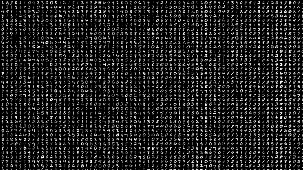
Similarly every algorithm in Machine Learning starts with a better dataset with as many as possible images of an object, so if we want to train an algorithm to predict a possibility of “0” or not a “0”, we need as much as possible handwritten “0s” to train our algorithm

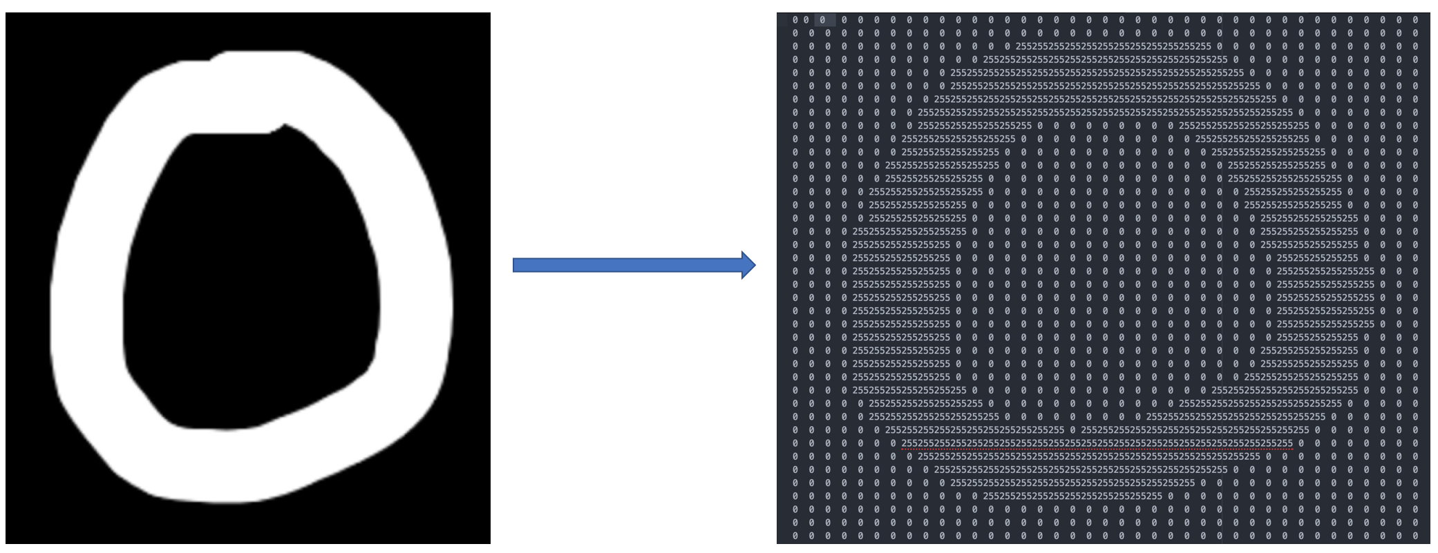
As I have talked about it in my last note, human brain can understand these image as it is trained over 500 million years but what about machines, the answer is incredibly simple – it is “0s” and “1s” but what about machine learning algorithms – A neural network takes numbers as input to a machine, an image is really just a grid of numbers that represents every pixel between 0 to 225. Why?
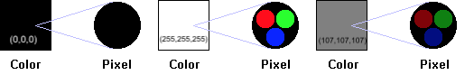
Here is the answer – each pixel on a computer screen is composed of three small dots of compounds called phosphors surrounded by a black mask. The phosphors emit light when struck by the electron beams produced by the electron guns at the rear of the tube. The three separate phosphors produce red, green, and blue light, respectively.
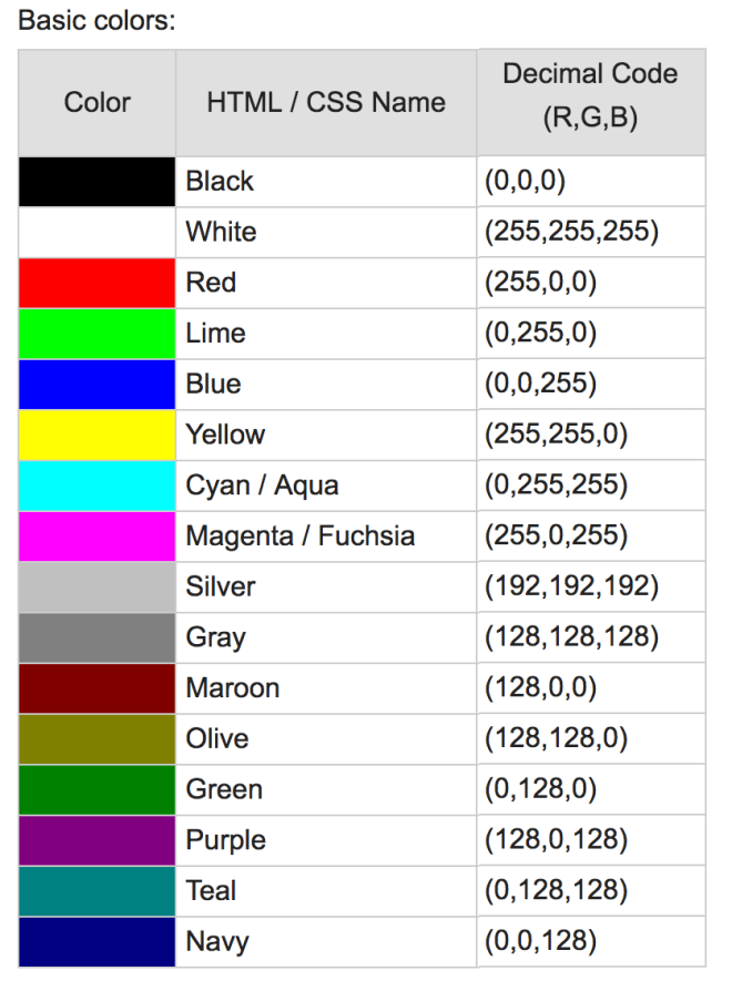
Channel is a conventional term used to refer to a certain component of an image. An image from a standard digital camera will have three channels – red, green and blue
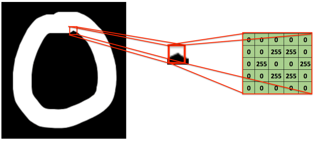
A grayscale image, on the other hand, has just one channel. For better understanding, lets take a grayscale images, we will have a single 2d matrix representing that image. The value of each pixel in the matrix will range from 0 to 255 – zero indicating black and 255 indicating white.
For algorithms, every pixel is a number, if it is a color image then following formula will work to convert it into grayscale image
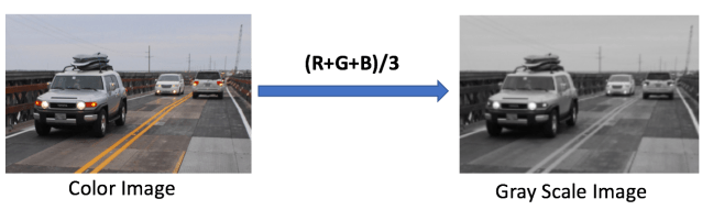
Note : R = Red, G = Green and B=Blue
To feed an image into our neural network, machine will take a train image and compute as grid with number e.g. as per following image
Train an algorithm
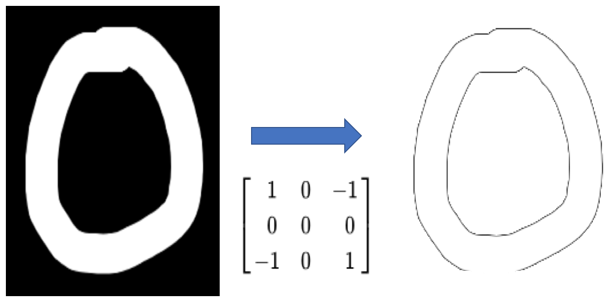
ConvNets derive their name from the “convolution” operator. The primary purpose of Convolution in case of a ConvNet is to extract features from the input image. Convolution preserves the spatial relationship between pixels by learning image features using small squares (or pixel) of input data. going to display some very common feature extraction with deep mathematical understanding.
Lets take a small grayscale image with (5 x 5) pixel values, as this is grayscale pixel color range will be in between 0 to 255.
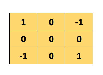
consider another other small image with (3 x 3) pixel values, why?
Here, this 3×3 matrix is called a ‘’filter’ or ‘kernel’ or ‘feature detector’ and the matrix formed by sliding the filter over the image and computing the dot product is called the ‘Convolved Feature’ or ‘Activation Map’ or the ‘Feature Map’.
Now, the Convolution of the 5 x 5 image and the 3 x 3 matrix can be computed as shown below
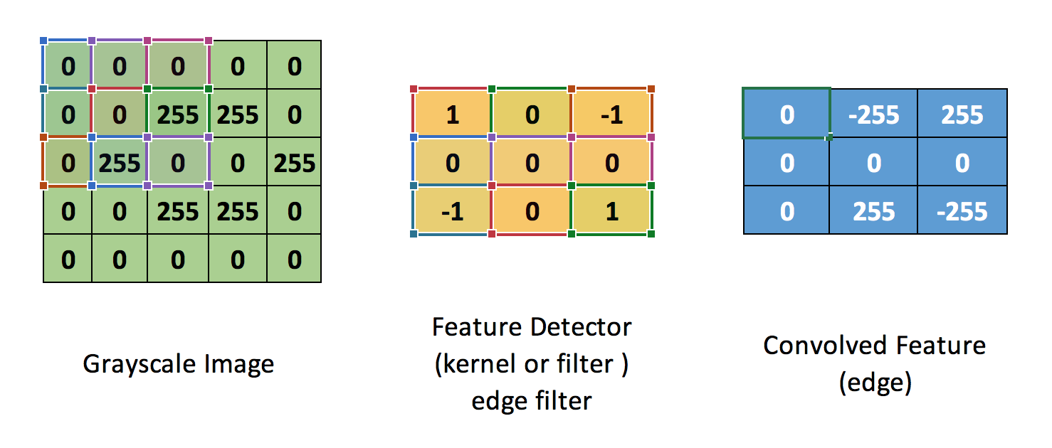
The output matrix is called Convolved Feature or Feature Map
Another way to understand this Convolution operation is by looking at the below animation
Lets understand how this computation above is being done. Slide the 3×3 matrix over our 5×5 input image (zero) by 1 pixel (also called ‘stride’) and for every position, compute element wise multiplication (between the two matrices) and add the multiplication outputs to get the final integer which forms a single element of the output matrix (Convolved Feature). and computation formula is
C[m,n] = ∑u∑υA[m+u,n+υ]⋅B[u,υ]
Convolved Feature
Now, we understand the analogy behind this process, lets consider our Zero image for the computation
Another good way to understand the Convolution operation, here are some example and demo for reference
http://matlabtricks.com/post-5/3×3-convolution-kernels-with-online-demo
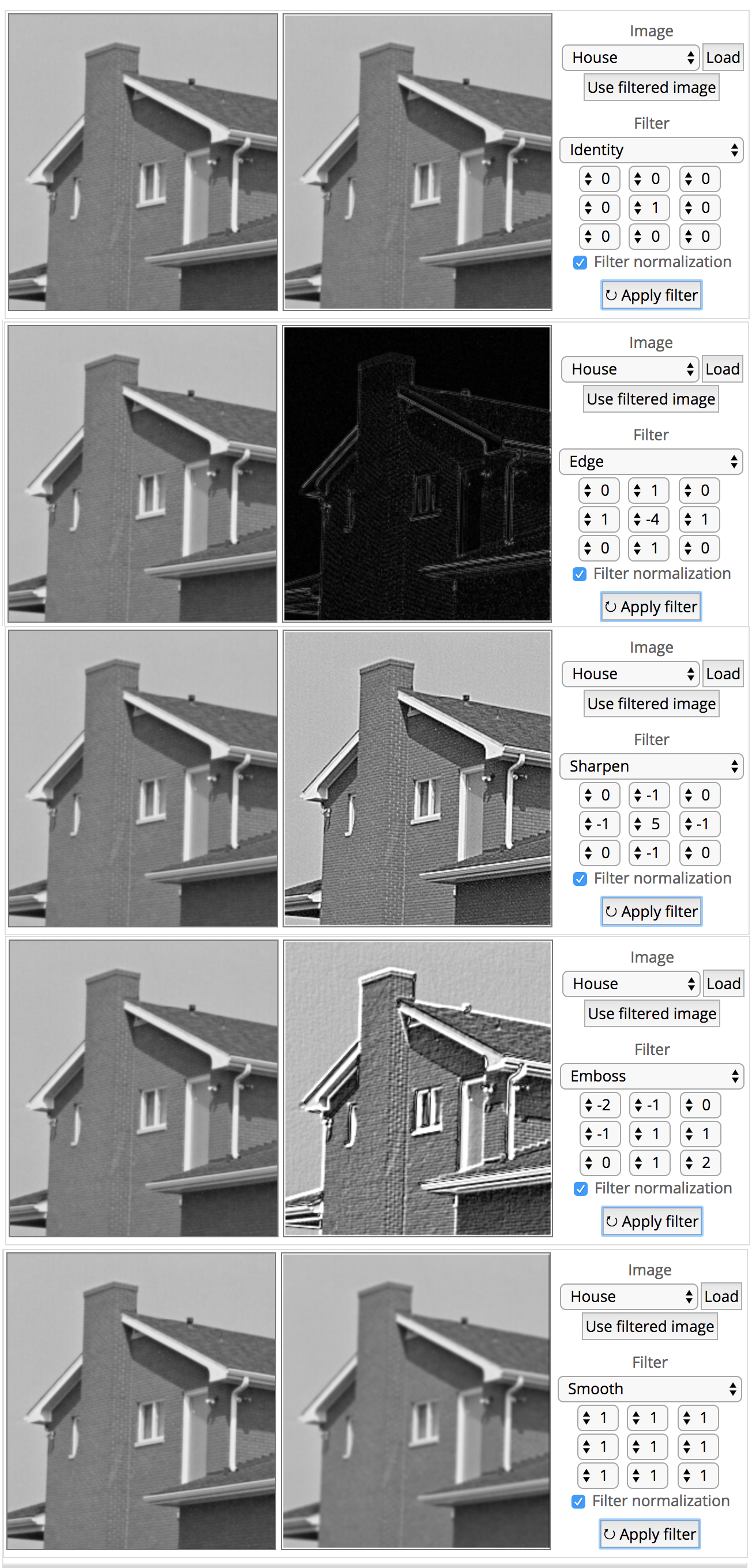
In reality, a ConvNets learns the values of applied filters on itself during the training process (although required number of filters, filter size, architecture of the network before hand).
Read more about these parameters (i.e. depth, Stride and Zero Padding) in my next note…
More number of filters means, more image features get extracted and the better network becomes at recognising patterns in unseen images.
Finally lets apply ConvNets with training process
More filters means, more intermediate layer using CNN to get finally fully connected layer
In my last note Autopilot – we saw that Convolution, ReLU and Pooling work. It is important to understand that these layers are the basic building blocks of any CNN. These layers extract the useful features from the images, introduce non-linearity in network and reduce feature dimension while aiming to make the features somewhat equivalent to scale and translation
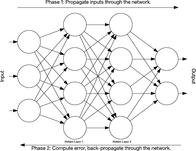
The overall training process of the Convolution Network is
- Start with, Initialising all filters and parameters / weights with random values
- The network takes a training image as input, processes it using forward propagation step (convolution, ReLU and pooling operations along with forward propagation in the Fully Connected layer) and finds the output probabilities for each class.
- Calculate the total error at the output layer Error = ∑ ½ (target probability – output probability) ²
- Error correction or Back propagation to calculate the gradients of the error with respect to all weights in the network and use gradient descent to update all filter values / weights and parameter values to minimise the output error.
- Repeat above steps with all images in the training set.
The above steps train the ConvNet – this essentially means that all the weights and parameters of the ConvNet have now been optimized to correctly classify images from the training set.
When start test dataset with new (unseen) images as input into the ConvNet, the network would go through the forward propagation step and output with a probability for each class. If training set is large enough, the network will generalize well to new images and classify them into correct categories.
Adam Harley created amazing visualizations of a Convolutional Neural Network trained on the MNIST Database of handwritten digits.
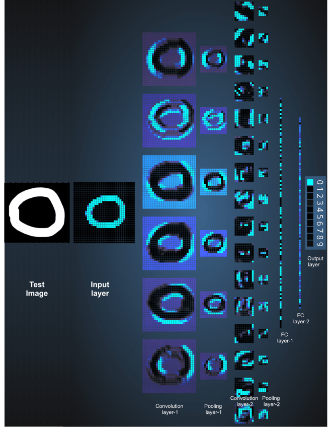
The test input image contains 1024 pixels (32 x 32 image) and the first Convolution layer is formed by convolution of six unique 5 × 5 (stride 1) filters with the test image. using six different filters produces a feature map of depth six.
Convolutional Layer 1 is followed by Pooling Layer 1 that does 2 × 2 max pooling (with stride 2) separately over the six feature maps in Convolution Layer 1.
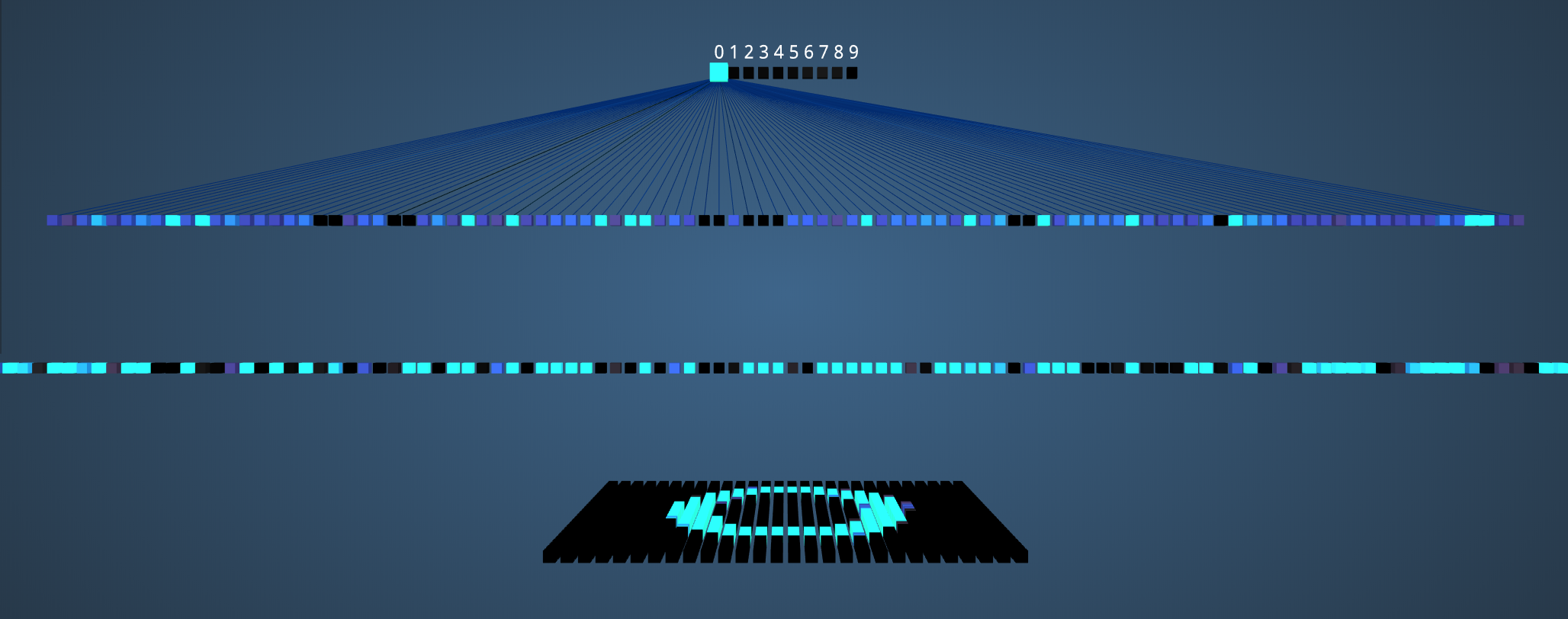
This process generates three fully-connected (FC) layers
- 120 neurons in the first FC1 layer
- 100 neurons in the second FC2 layer
- 10 neurons in the third FC3 layer corresponding to the 10 digits – also called the Output layer
Okay, now we are able to understand what is happening behind the screens, lets start with our original question “How apps are doing on phone? “
Every Photos Apps (e.g. iPhone’s Photos, Google Photos and Facebook) allows users to back up their photos from multiple devices in a single location including photo/video sharing and storage service, Google Photos includes unlimited photo and video storage, and apps for Android, iOS, and the browser. Users back up their photos to the cloud service, which become accessible between all of their devices connected to the service.
Recently, using this photos and videos Apps introduced creates an album that collect photos taken during a specific period organized into an album of showing the “best” photos from the trip, event, and location. In order to identify the “best” photos, the app uses machine learning where a computer has been trained to “learn” to recognize images.
These storage and images from user works as Training Dataset to Deep Learning Algorithm before it will start predicting for us on Phone. It is called Test data and ratio between train vs test is 70/30.
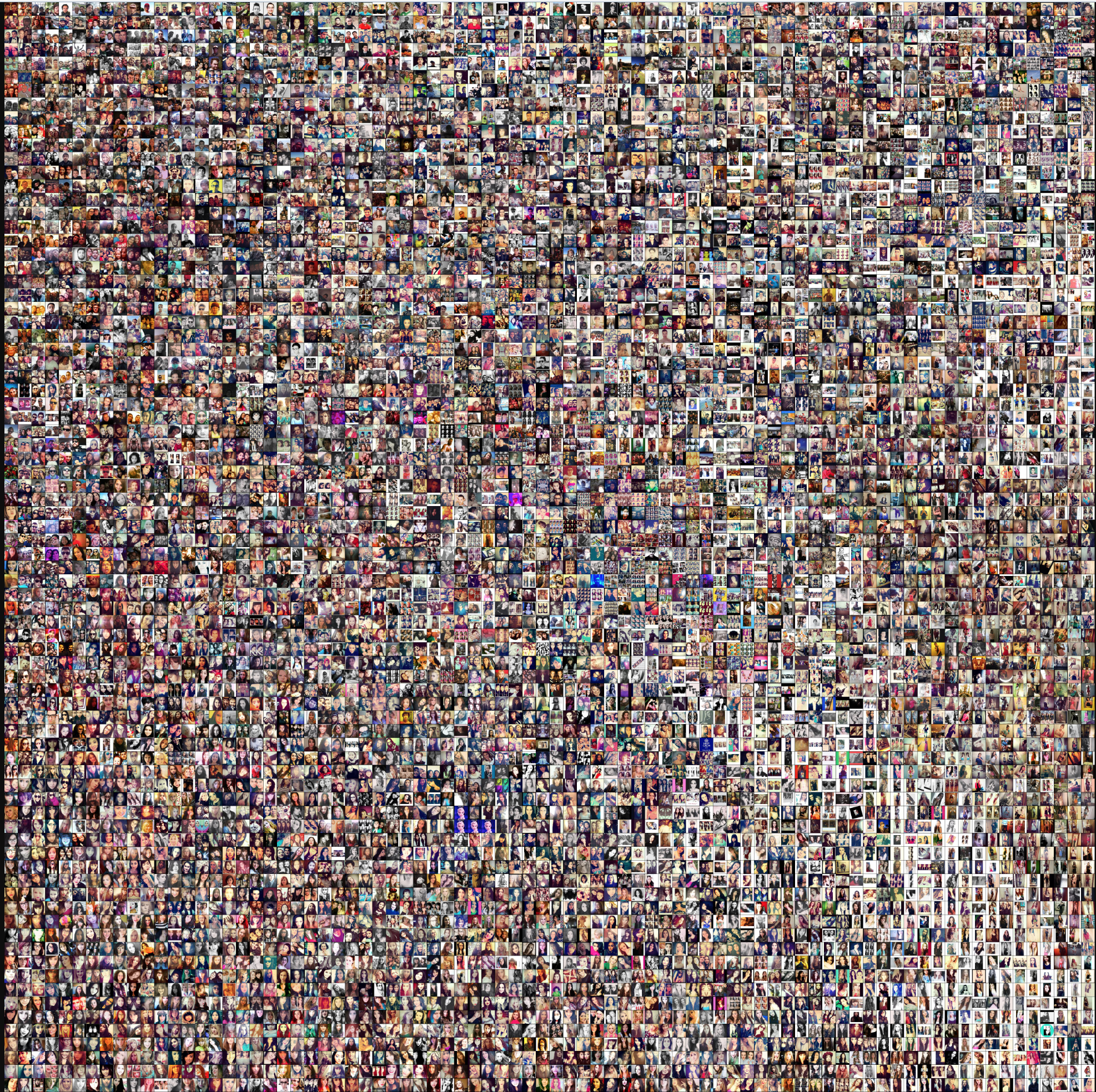
Here is a link to a higher-resolution version. (9MB)
Summary
Convolutional Neural Networks is good to recognise things, places and people in photos, signs, people and lights in self-driving cars, crops, forests and traffic in aerial imagery, various anomalies in medical images and all kinds of other useful things.
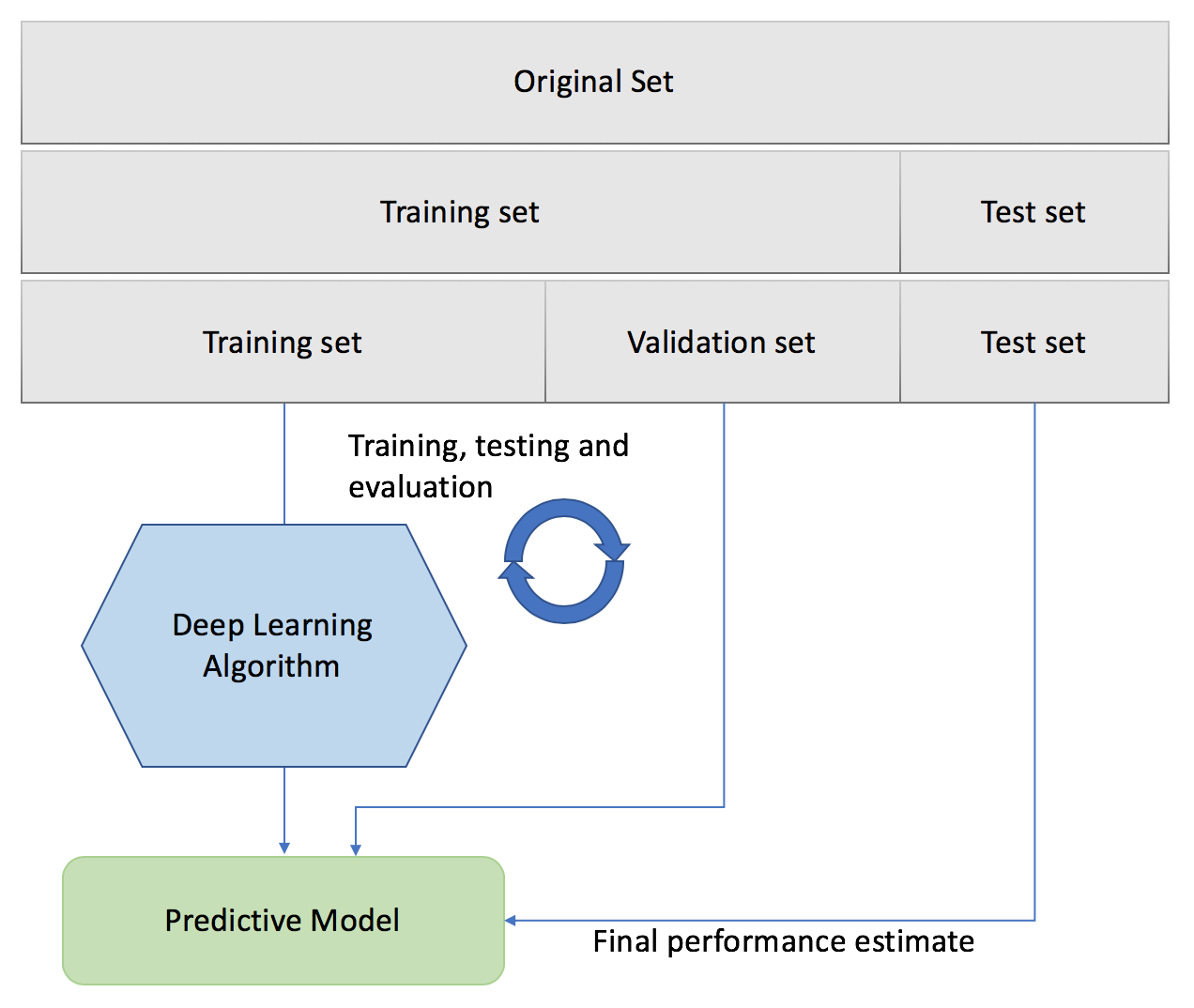
But most important part is Training a model, there are 2 type of datasets
- In one dataset (“gold standard”), have the input data together with correct/expected output, This dataset is usually duly prepared either by humans or by collecting some data in semi-automated way. But it is important that it have the expected output for every data row here.
- 2nd data we are going to apply in model. In many cases this is the data in which we are interested for the output of our model.
While performing Convolutional Neural Networks
- Training phase: we present our data from our “gold standard” and train our model, by pairing the input with expected output.
- Validation/Test phase: in order to estimate how well our model has been trained (that is dependent upon the size of data, the value we would like to predict, input etc) and to estimate model properties (mean error for numeric predictors, classification errors for classifiers, number of filers etc.)
- Testing phase: now we apply our freshly-developed model to the real-world data and get the results.
In this note, I have tried to explain deep learning with very common examples with train vs test process including some mathematics and complexity behind it.

Leave a comment