Audio Recognition with Deep Learning

Today, in this note lets discuss about audio recognition, but before that we will talk about it’s visualisation,

When we talk about Machine Learning, most of the examples out there are like image processing and Recommendation Engine, Loan Prediction problem and Fraud detection. I believe, the example discussed ahead is little different and complex.

Interestingly, an audio represents many unstructured data points. It is closer to how we communicate and interact as humans. It also contains a lot of useful & powerful information and from audio data we get the words, sentences and also emotions.

In this note, I will try to explain an overview of audio and sound structure and will focus on how to convert it in to an input for machine learning algorithm for classifying the audio. We will analyse audio and train a model to find all the spectrum and different sounds including human voice.

Let’s start with Audio and Sound Data

Directly or indirectly, we are always in contact with audio. Human brain is continuously processing and extracting useful information from the audio data it comes in contact with.

If some conversation is going on somewhere, then a Human brain listening to that conversation will process and extract following information

How many people are involved in the conversation?
Emotions like aggressiveness, motivation, depression and others
Sounds other than human voice like clock ticks or coffee machine sound …etc

A human brain is already trained enough to understand and analyse any sound but the question is how a machine does the same.

Directly or indirectly, we are always in contact with audio. Our brain is continuously processing and understanding audio data. Even when you are alone in a room in a quiet environment, you tend to catch much more subtle sounds, like the watch ticks, rain drops and many others.

Let’s start with Audio data structure; you might be thinking why?

The simplest way to answer this question is, a machine understand 0s, and 1s so in order for a machine to understand ,somehow we have to convert any image, signal and audio in numeric format comprised of 0s and 1s…please refer to my previous notes.

An audio is a pressure wave sampled at tens of thousands times per second and stored as an array of numbers.

Lets see how audio data looks like and stored in a file. We will focus on recognising spoken commands in following audio clip like this

Audio with single word “Hello”

The standard way of generating images from audio is by looking at the audio chunk-by-chunk, and analysing it in the frequency domain. Lets talk about some techniques to convert it.

Waveform plotted as pressure as a function of time

Waveform plotted as pressure for single word “Hello”

Preprocessing Audio Files

For audio classification, we have to compute either filter banks or MFCCs using following steps

A signal goes through a pre-emphasis filter
then gets sliced into (overlapping) frames and a window function is applied to each frame;
afterwards, apply Fourier transform on each frame (or more specifically a Short-Time Fourier Transform)
and calculate the power spectrum;
and subsequently compute the filter banks.
To obtain MFCCs, a Discrete Cosine Transform (DCT) is applied to the filter banks retaining a number of the resulting coefficients while the rest are discarded.

Pre-Emphasis

The first step is to apply a pre-emphasis filter on the signal to amplify the high frequencies. A pre-emphasis filter is useful in several ways

Balance the frequency spectrum since high frequencies usually have smaller magnitudes compared to lower frequencies,
Avoid numerical problems during the Fourier transform operation and
May also improve the Signal-to-Noise Ratio (SNR).

The pre-emphasis filter can be applied to a signal x using the first order filter in the following equation:

y(t)=x(t)−αx(t−1)

Output = Input – (PRE_EMPH_FACTOR * Previous_input)
here PRE_EMPH_FACTOR (a) as 0.975.

It depends on best overlap buffers to ensures that we don’t miss out any interesting details happening at the buffer boundaries.

Framing

After pre-emphasis, we have to split the signal into short-time frames. The rationale behind this step is that frequencies in a signal change over time, so in most cases it doesn’t make sense to do the Fourier transform across the entire signal in that we would loose the frequency contours of the signal over time. To avoid that, we can safely assume that frequencies in a signal are stationary over a very short period of time. Therefore, by doing a Fourier transform over this short-time frame, we can obtain a good approximation of the frequency contours of the signal by concatenating adjacent frames.

Short-time frames for single word “Hello”

Typical frame sizes in speech processing range from 20 ms to 40 ms with 50% (+/-10%) overlap between consecutive frames. Popular settings are 25 ms for the frame size, frame_size = 0.025 and a 10 ms stride (15 ms overlap

Fourier-Transform and Power Spectrum

We consider each frame in the frequency domain. We can do this using Fast Fourier Transform (FFT) algorithm.

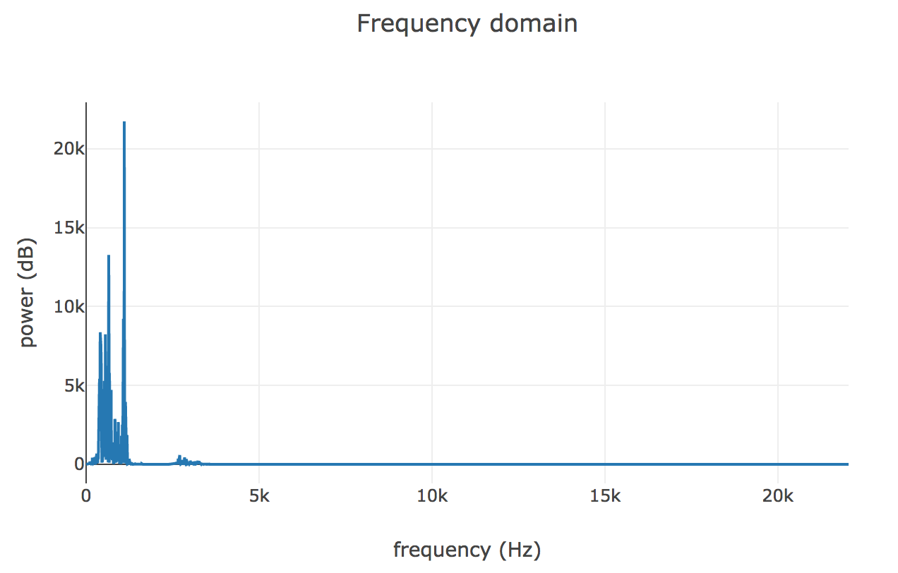
This algorithm gives us complex values from which we can extract magnitudes or energies. For example, here are the FFT energies of one of the buffers, approximately the second one in the above image, where the speaker begins saying the “he” syllable of “hello”.

Fast Fourier transform (FFT) is an algorithm that computes the discrete Fourier transform (DFT) of a sequence, or its inverse (IDFT). Fourier analysis converts a signal from its original domain (often time or space) to a representation in the frequency domain and vice versa.

Imagine we do this for every buffer we generated in the previous step, take each Fast Fourier Transform (FFT) array and instead of showing energy as a function of frequency, stack the array vertically so that y-axis represents frequency and color represents energy. This is called spectrogram.

An spectrogram is a visual representation of the spectrum of frequencies of sound or other signals as they vary with time. Spectrograms are sometimes called sonographs, voiceprints, or voicegrams. When the data is represented in a 3D plot they may be called waterfalls.

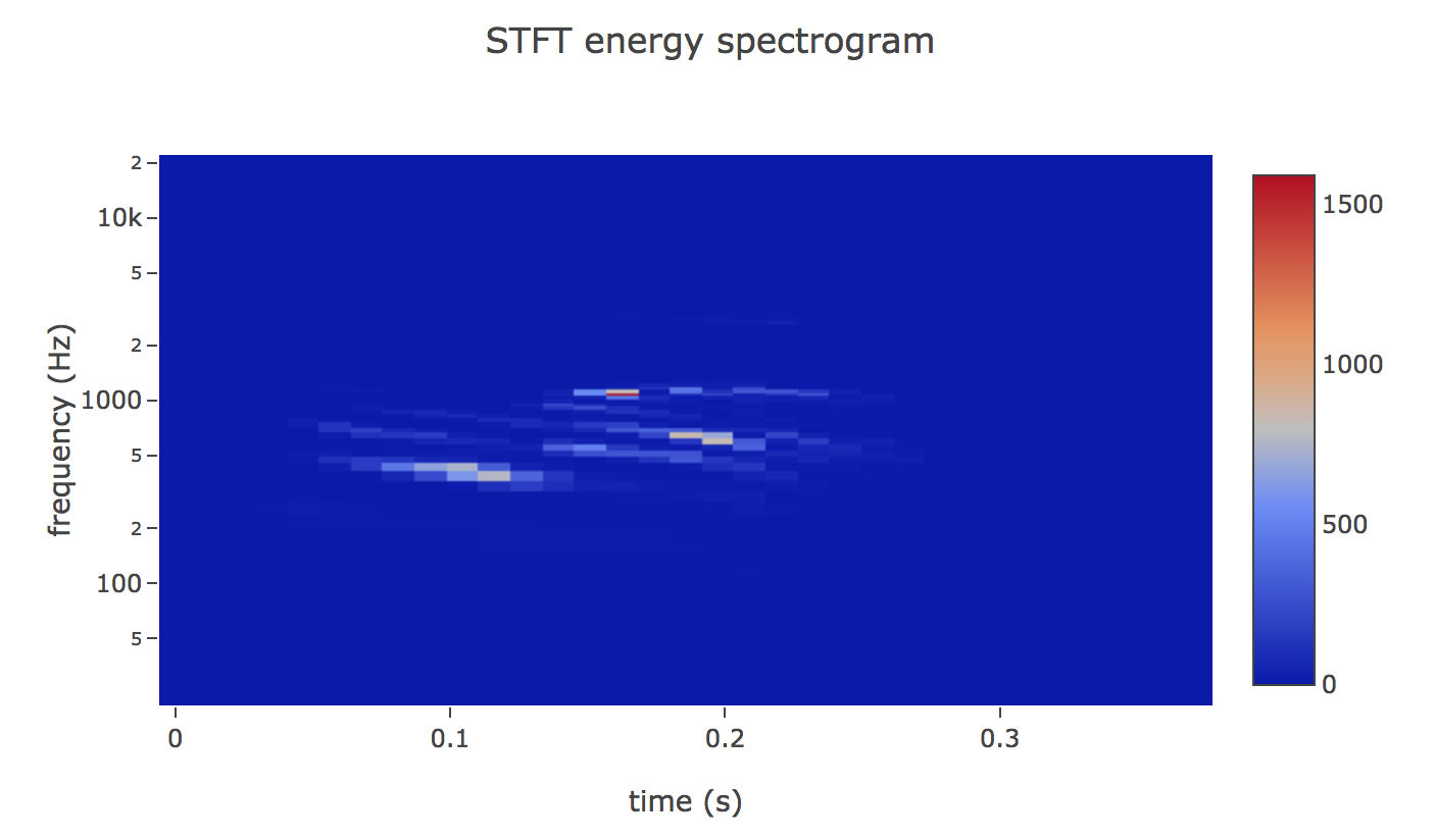
STFT energy spectrogram for single word “Hello”

We could use this image into our neural network (CNN), but it looks pretty sparse as it has wasted so much space, and there’s not much signal there for a neural network to train on.

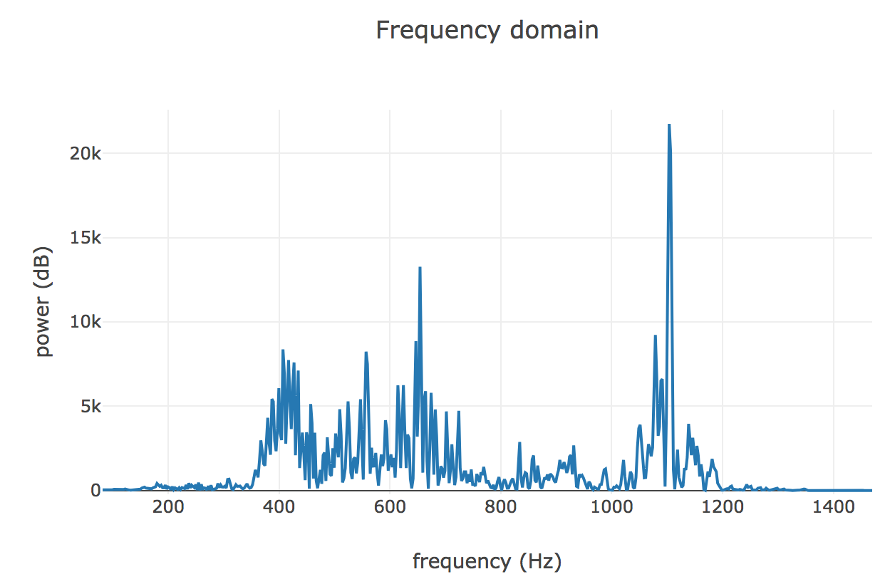
Let’s go back to the Fast Fourier Transform (FFT) plot to zoom our image into our area of interest. The frequencies in this plot are bunched up below 5 KHz since the speaker isn’t producing particularily high frequency sound. Human audition tends to be logarithmic, so we can view the same range on a log-plot

Filter Banks

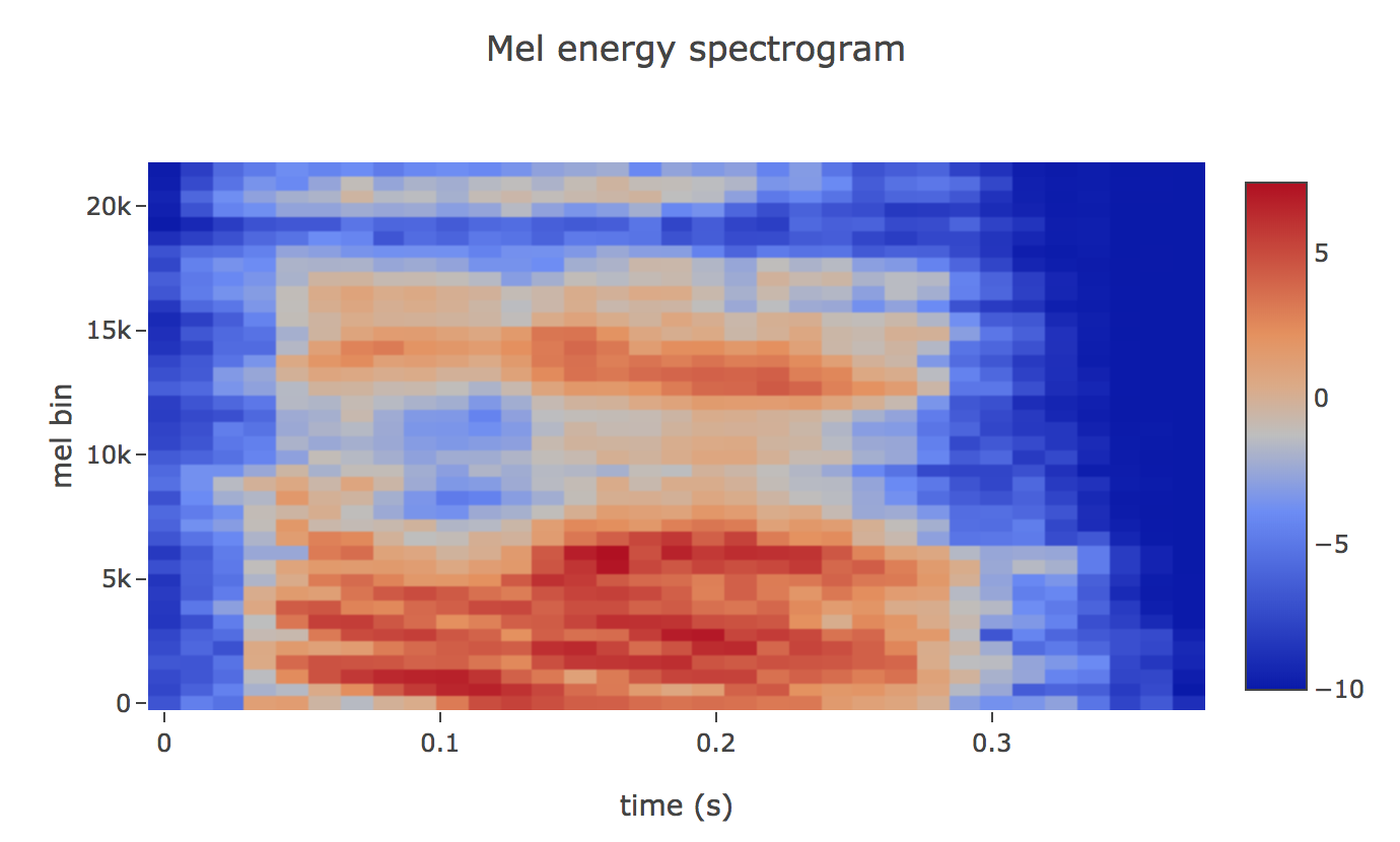
Humans are much better at discerning small changes in pitch at low frequencies than at high frequencies. The Mel scale relates pitch of a pure tone to its actual measured frequency. To go from frequencies to Mels, we create a triangular filter bank

The final step to computing filter banks is applying triangular filters, typically 40 filters, nfilt = 40 on a Mel-scale to the power spectrum to extract frequency bands. The Mel-scale aims to mimic the non-linear human ear perception of sound, by being more discriminative at lower frequencies and less discriminative at higher frequencies. We can convert between Hertz (f) and Mel (m) using the following equations

Mel (m)=2595log10(1+f700)

frequency (f)=700(10m/2595−1)

Plotting this as an spectrogram, the log-mel spectrogram to get the feature

If the Mel-scaled filter banks were the desired features then we can skip to mean normalization.

Mel-frequency Cepstral Coefficients (MFCCs)

It turns out that filter bank coefficients computed in the previous step are highly correlated, which could be problematic in some machine learning algorithms. Therefore, we can apply Discrete Cosine Transform (DCT) to decorrelate the filter bank coefficients and yield a compressed representation of the filter banks.

MFCC spectrogram for single word “Hello”

One may apply sinusoidal liftering to the MFCCs to de-emphasize higher MFCCs which has been claimed to improve speech recognition in noisy signals.

Filter Banks vs MFCCs

It is interesting to note that all steps needed to compute filter banks were motivated by the nature of the speech signal and the human perception of such signals.

On the contrary, the extra steps needed to compute MFCCs were motivated by the limitation of some machine learning algorithms.
And MFCCs were very popular when Gaussian Mixture Models – Hidden Markov Models (GMMs-HMMs) were very popular and together.

Summary

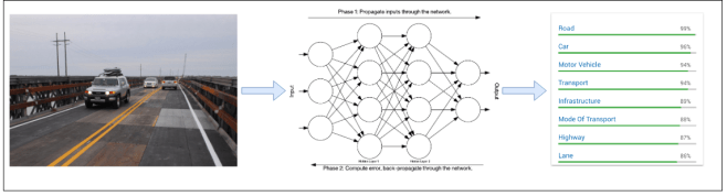
Convolutional Neural Networks (CNNs) are a big reason why there has been so much interesting work done in computer vision recently. CNN networks is designed to work on matrices representing 2D images.

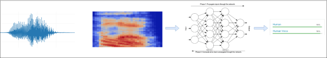
So if we want to use CNN to classify sound then have to convert audio to image and apply CNN network.

Machine Learning for vision

Machine Learning for hearing

In next note, I will go in deep on how to reduce noise, apply CNN on Audio and classify the different voices, and extract other sounds.

Please read my previous notes: